With so much data📚 gathered in the corporate sector, we must now have some methods of painting🎨🖌 an image of that information to comprehend it. Data analysis📊 enables us to understand the data and identify trends, patterns📈. We can now achieve all the above-said things by the techniques used in Data Science, thanks to Python's Pandas library! 🌟

Pandas is data manipulation and analysis library written using Python. It has a plethora of functions and methods to help speed up⚡ the data analysis process. Pandas’ popularity stems from its usefulness, adaptability, and straightforward syntax🤩.

Over the years, Pandas has been the industry standard🏭 for data reading and processing. This blog includes the top ten Pandas techniques that will be more than useful in your data science projects.💯

How to start with Data structures & Algorithms

1. Conditional Selection of Rows

Exploratory Data Analysis is done to summarise the key🗝 characteristics and to better understand the data set📋. It also helps us rapidly evaluate the data and experiment with different factors to see how they affect the results. One of the important analyses is the conditional selection of rows or data filtering. There are two methods to do this.

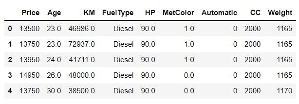
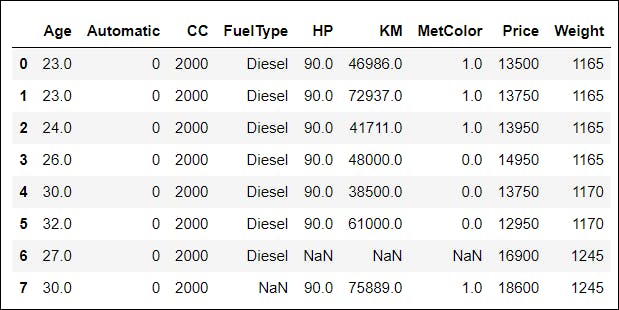
📌 The examples shown below utilizes a data set that specifies different properties of cars🚘. Take a look at the data set:

import pandas as pd
path = "C:/Users/aakua/OneDrive/Desktop/Toyota.csv"

df = pd.read_csv(path,na_values=["??","###","????"], index_col=0)
df.head()

Output:

a. loc[ ]

The Pandas DataFrame.loc[] property allows you to access a set of rows and columns in the supplied data set by label(s) or a boolean array.

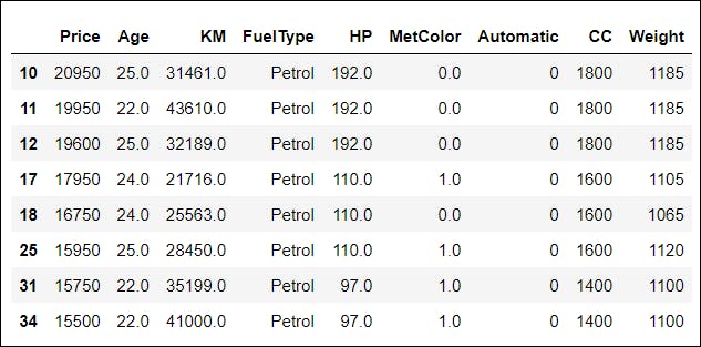
📌 For this example, we will filter the rows with Age <=25 and FuelType as Petrol.

data = df.loc[(df['Age'] <= 25) & (df['FuelType'] == 'Petrol')]
data[:8]

Output:

b. query( )

The query( ) method is used to query the columns of a DataFrame with a boolean expression.🌟The only significant difference between a query and a standard conditional mask is that a string can be regarded as a conditional statement in a query. In contrast, a conditional mask filters the data with booleans and returns the values according to actual conditions.

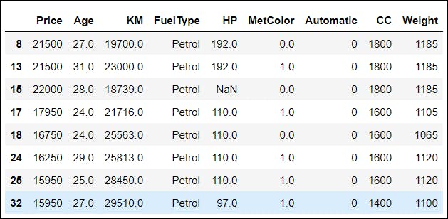
📌 Here, we have filtered the rows that have KM values between 15000 and 30000.

data_q = df.query('15000.0 < KM < 30000.0')
data_q[:8]

2. Sorting

Pandas provide two methods for sorting the data frame: sort_values( ) and sort_index( ). 🚩The sorting order can be controlled.

a. sort_values( ):

This function is used to sort one or more columns of the Pandas DataFrame. We have sorted the data frame in ascending order according to the Price column.

df.sort_values(by = 'Price')[:8]

Output:

b. sort_index( ):

This is used for sorting Pandas DataFrame by the row index.

df.sort_index(axis=1, ascending = True)[:8]

Output:

3. GroupBy

A GroupBy operation involves some combination of splitting the object, applying a function, and combining the results. It may be used for grouping vast quantities and computing operations on them.

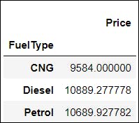
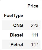
📌 A. Let us say we want to look at the average price of the cars according to different FuelType, such as CNG, Petrol and Diesel. Take a moment and think about the problem🤔.

GroupBy function can quickly implement this! We will first split the data according to the FuelType, and then apply the mean( ) function to the price.

df.groupby(['FuelType'])[['Price']].mean()

Output:

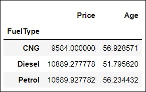
📌 B. Now, we will group the data as before, but we will also compute the mean of the Age of cars.

df.groupby(['FuelType'])[['Price', 'Age']].mean()

Output:

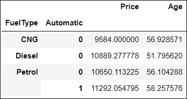
📌 C. What if you want to group the data according to more than one column?🧐 Here’s the solution:

df.groupby(['FuelType','Automatic'])[['Price', 'Age']].mean()

Output:

See, that was easy!😉 Let us explore the next one now.

4. Mapping

Another essential data manipulating technique is data mapping. Initially, as a mathematical concept, mapping is the act of producing a new collection of values, generally individually, from an existing set of values. 🌟The biggest advantage of this function is that it can be applied to an entire data set.📚

The Pandas library offers us the map() method to handle series data. For mapping one value in a set to another value depending on input correspondence, Pandas map() is employed. This input may be a series or even a dictionary.

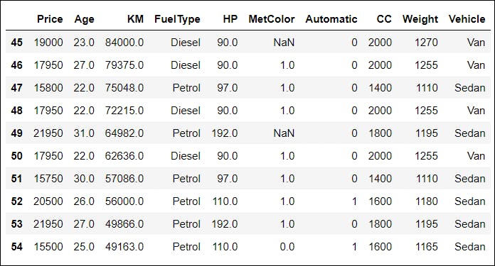
📌 Let us map the FuelType variable with Vehicle Type. For instance, CNG will be mapped with Hatchback, Petrol with Sedan, and Diesel with Van.

# dictionary to map FuelType with Vehicle
map_fueltype_to_vehicle = { 'CNG' : 'Hatchback', 
                  'Petrol' : 'Sedan', 
                  'Diesel' : 'Van'}

df['Vehicle'] = df['FuelType'].map(map_fueltype_to_vehicle)
df[45:55]

Output:

5. nsmallest( ) and nlargest( )

I think, after reading their titles, there is no doubt about the goals🎯 of these two approaches; nonetheless, here are the definitions:

a. nsmallest( ): The Pandas nsmallest( ) technique is used to obtain n least👇 values in the data set or series.

b. nlargest( ): The Pandas nlargest( ) function obtains n largest👆 values in the data set or series.

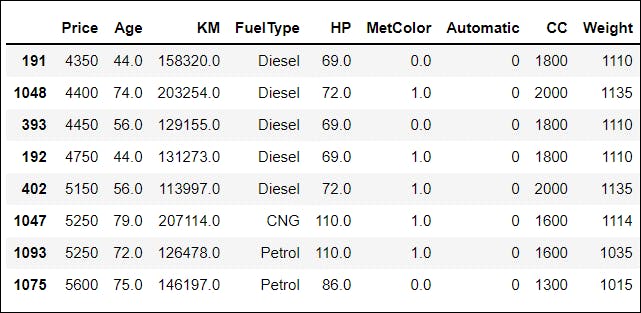
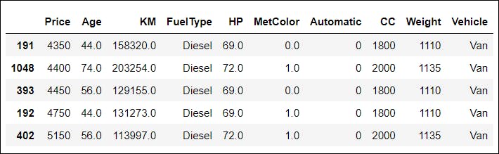
📌 Let us examine how the five observations with the least and most value would be found in the Price column:

df.nsmallest(5, "Price")

Output:

df.nlargest(5, "Price")

Output:

6. idxmax( ) and idxmin( )

a. idxmax( ): Pandas DataFrame.idxmax( ) gives the index of the first occurrence of maximum value across the specified axis. All NA/null values are omitted❌ when determining the index of the greatest value across any index.

b. idxmin( ): Pandas DataFrame.idxmin( ) gives the index of the first occurrence of minimum value across the specified axis. All NA/null values are omitted ❌ when determining the index of the least value across any index.

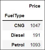
📌 Let us say we want to access the indices of the maximum and minimum values in the Price column based on the FuelType. This can be done in the following manner:

df.groupby(['FuelType'])[['Price']].idxmin()

Output:

df.groupby(['FuelType'])[['Price']].idxmax()

Output:

7. Exporting Data

While performing different functions on the data set, as explained above, grouping data becomes helpful. However, what if we want to save the grouped data as a new file in our system? 🤔🧐

Pandas offer functions that can come in handy in such situations🌟, that can save a DataFrame as a file in various extensions like .xlsx, .csv, etc.

data_q = df.query('15000.0 < KM < 30000.0')
data_q.to_csv('Query_Data.csv')

Output: File Saved

📌 To save the data frame in Excel use: to_excel( )

📌 To save the data frame in JSON use: to_json( )

8. dropna( ) and fillna( )

The data set sometimes includes null values✖ that are shown in the DataFrame as NaN afterward.

a. dropna( ): The dropna( ) method in Pandas DataFrame is used to eliminate❌ rows and columns containing Null/NaN values.

df.shape

Output: (1436, 9)

data1 = df.dropna()
data1.shape

Output: (1097, 10)

b. fillna( ): fillna( ), unlike the pandas dropna( ) method, handles and removes❌ Null values from a DataFrame by allowing the user to substitute NaN values with their own.

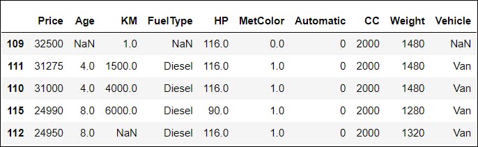
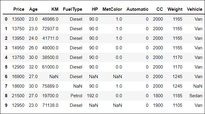
📌 Before eliminating null values, the data set looked like:

df.head(10)

Output:

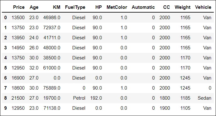
📌 I have substituted the null values with 0. After using the fillna( ) method:

df = df.fillna(0)
df.head(10)

Output:

9. Correlation

Pandas DataFrame.corr( ) returns the pairwise correlation of all columns in a DataFrame. Any NA values are immediately filtered out. It is disregarded for any non-numeric data type columns in the DataFrame.

df.corr()

Output:

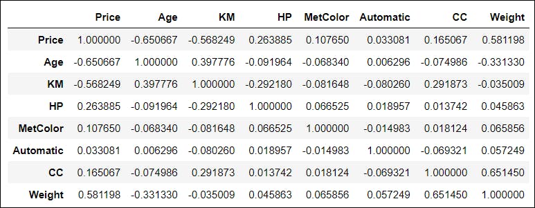
🚩Some key points to note about correlation values:

📍 The correlation values fluctuate between -1 and 1.

📍 1 implies that the association is 1 to 1 (perfect correlation), and one value in the second column has risen every time a value has been increased in the first column.

📍 0.9 indicates a strong connection, and the other is similarly likely to rise if you increase one value.

📍 -0.9 would be exactly as good as 0.9, but the other would definitely decrease if you increase one value.

📍 0.2 does NOT imply a good correlation, which means that if one value goes up does not imply the other goes up too.

📍 I believe, it is reasonable to claim that the two columns have a decent correlation if the values are between -0.6 and 0.6.

10. Apply a function to the DataFrame

The apply( ) function is used to implement arithmetic or logical code over an entire data set or series type using a Python function. The function to be applied can be an inbuilt function or a user-defined function.

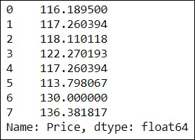
a. Applying an inbuilt function:

import numpy as np
df['Price'].apply(np.sqrt)[:8]

Output:

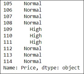
b. Applying a user-defined function:

def fun(num):

    if num <10000:
        return "Low"

    elif num >= 10000 and num <25000:
        return "Normal"

    else:
        return "High"


new = df['Price'].apply(fun)
new[105:115]

Output:

You will surely have the advantage of knowing these approaches from Pandas in the field of data science🤩. I hope you liked and found this blog useful!🌟

Read our latest blogs...

Python Pandas for beginners

Subscribe to our YouTube channel for more great videos and projects.