Dijkstra’s vs. A* Search Algorithm
An introduction to two well-known path-finding algorithms and a comparison of them by analyzing each one with an example.
If you love to code and have solved interview questions of the FAANG companies, you would have realized that in many of these puzzles, various graphs seem to apply the same logic, consciously you feel that YES,🔰 you know the answer or at least the approach, and yet you fail to solve them. 😞
Today in this blog, we will discuss two of the most commonly used path-finding algorithms to solve Graph Traversal Problems:
- 📍 Dijkstra’s Algorithm to find the shortest path between any two graph nodes
- 📍 A* search Algorithm to find a path in a game-like scenario.
💡 Remember that to a given problem both these approaches might fit; now it’s up to you to choose the approach you are most confident about. Knowing both methods come in handy, especially when for a given problem, there exist time constraints - one algorithm meets the time constraint✔️ while the other doesn’t.❌ So, let’s get started!
In this blog, I will try to cover the following topics:
|-- Dijkstra’s Algorithm
| -- Basic Concepts
| -- Algorithmic Steps
| -- Implementation in Python
| -- A* Search Algorithm
| -- Basic Concepts
| -- Heuristics
| -- Algorithmic Steps
| -- Implementation in Python
| -- Comparison between these two algorithms
Weigh your thoughts with Graphs!
Before we can really dive into Dijkstra's Famous Algorithm, we need to gather a few seeds of vital information that we'll need along the way.📝 It's finally time for us to meet the Weighted Graph! A weighted graph is intriguing since it is unaffected by whether the graph is directed or undirected or whether it contains cycles.
At its most basic level, a weighted graph is a graph with edges that have some form of value associated with them. The “weight” of an edge is determined by the value attributed to it. The cost or distance between two nodes is a common way of referring to the "weight" of a single edge.
Now, the weight of a graph begins to complicate things slightly here;🚧 finding the shortest path between two nodes becomes considerably more complicated when we have to account for the weights of the edges we are traversing.
Do you believe that finding the shortest path between nodes using the Brute-Force Method would be Viable, Scalable, and Efficient when dealing with large trees, say, 20 nodes⁉️ The explanation is that it isn't realistic nor is it really any fun!👎And that’s where Dijkstra comes to the rescue.💪
Dijkstra's Shortest Path Algorithm
Dijkstra’s Algorithm and Its Basic Concepts
Dijkstra's Algorithm is special for various reasons, which we'll discover as we learn more about how it works.🌟 But the fact that this approach isn't merely utilized to identify the shortest path between two specified nodes in a graph data structure has always caught me off guard.💁
Dijkstra's Algorithm can be used to find the shortest path between any two nodes in a network, as long as the nodes are reachable from the beginning node.
📍 This algorithm will continue to run until all of the reachable vertices in a graph have been visited. This implies we could use Dijkstra's Algorithm to identify the shortest path between any two reachable nodes and save the results somewhere.📋 We can run Dijkstra’s Algorithm just once and look up our results from our algorithm again and again, without having to actually run the algorithm itself!🙌
The only time we'd need to re-run Dijkstra's Algorithm is if something about our graph data structure changed, in which case we'd need to do so to guarantee that we still have the most up-to-date shortest paths for our data structure.✔️
Path-finding issues, such as detecting directions or finding a route on Google Maps, are the most common application of Dijkstra's Algorithm.🚩 To identify a path through Google Maps, however, implementation of Dijkstra's Algorithm must be considerably more clever, taking into account a weighted graph and traffic, road conditions, road closures, and construction.🎯
Alright! Do not worry if all of this seems overwhelming!😅 The following section will undoubtedly ease your mind.👇❄️
Behind the scenes of Dijkstra’s Algorithm
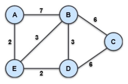
Let's consider an Undirected, Weighted Graph shown below:

📌Let's assume we're looking for the shortest route between nodes A and C.
👉 We know we'll start at node A, but we have no idea if there is a path to get there or if there are several paths! In any scenario, we have no idea which path will be the shortest to go to node C, assuming one exists at all.
Before we go any further, let's go over the process for using Dijkstra's Algorithm.
- 📍 Every time we set out to visit a new node, we will prioritize visiting the node with the shortest known distance/cost.
- 📍 We'll inspect each of its nearby nodes once we've arrived at the node we're going to visit.
- 📍 We'll determine the distance/cost for each surrounding node by adding the costs of the edges that lead to the node we're checking from the starting vertex for each neighboring node.
- 📍 Finally, if the distance/cost to a node is less than a known distance, the shortest distance we have on file for that vertex will be updated.
📌 Now, let's get started with our example!
💡Step 1: Inspecting the nearby nodes of the starting node A
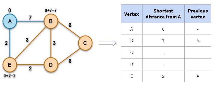
💡Step 2: Update the value if a shorter path is found

💡Step 3: Update the value if a shorter path is found and calculate all the remaining paths
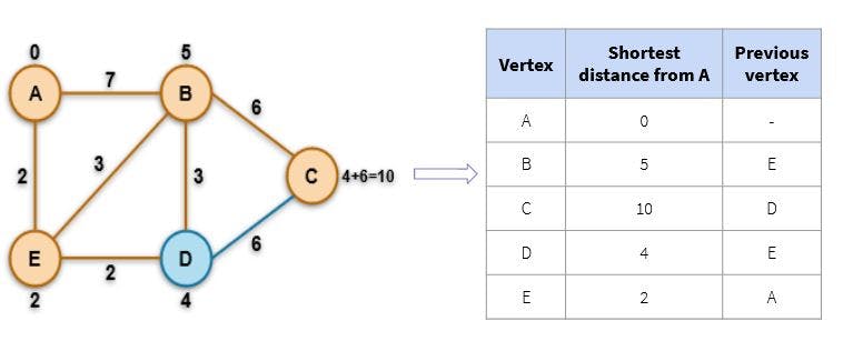
Tracing our paths now, the exact path that gives us the shortest distance between the nodes
AandCis:A -- E -- D -- C.
Any shortest path in this table can be found by retracing our steps and returning to the initial node by following the “previous vertex” of any node. 🔃
Let's suppose we decide that we want to locate the shortest path from point A to point D. We don't need to run Dijkstra's Algorithm again because we already have all we need right here!✔️
We’ll start with node D, then look at node D's previous ↩️ vertex, which happens to be node E. Similarly, we’ll look at node E's previous vertex which is node A, our starting vertex! Once we trace our steps all the way back up to our starting vertex,🔄 we can get the results in this order: A -- E -- D. As it turns out, this is the exact path that gives us the lowest cost/distance from node A to node D!🙌
Implementation with Python
nodes = ('A', 'B', 'C', 'D', 'E')
distances = {
    'B': {'A': 7, 'C': 6, 'D': 3, 'E': 3},
    'A': {'B': 7, 'E': 2},
    'C': {'B': 6, 'D': 6},
    'D': {'B': 3, 'C': 6, 'E': 2},
    'E': {'A': 2, 'B': 3, 'D': 2}}

unvisited = {node: None for node in nodes} #using None as +inf
visited = {}
current = 'A'
currentDistance = 0
unvisited[current] = currentDistance
while True:
    for neighbour, distance in distances[current].items():
        if neighbour not in unvisited:
            continue
        newDistance = currentDistance + distance
        if unvisited[neighbour] is None or unvisited[neighbour] > newDistance:
            unvisited[neighbour] = newDistance
    visited[current] = currentDistance
    del unvisited[current]
    if not unvisited:
        break
    candidates = [node for node in unvisited.items() if node[1]]
    current, currentDistance = sorted(candidates, key = lambda x: x[1])[0]
print(visited)
Output:
{'A': 0, 'E': 2, 'D': 4, 'B': 5, 'C': 10}
A* Search Algorithm
A* Algorithm and Its Basic Concepts
The most important advantage of the A* Search Algorithm, which separates it from other traversal techniques, is that it has a brain!!🧠 This makes A* very smart and pushes it much ahead of other conventional algorithms.👑
Actually, the A* Search Algorithm is built on the principles of Dijkstra’s Shortest Path Algorithm itself but provides a faster solution 🚀 when faced with finding the shortest path between two nodes.
It accomplishes this by incorporating a heuristic element that helps select the next node to examine as the path progresses.
Heuristic Function
(A simple mathematical expression but with a complicated name!😆)
Remember you read in the earlier context about the A* Algorithm having a brain?🧠 This is it! The A* Algorithm employs a heuristic function to assess and analyze which path to take next.💭 The heuristic function calculates the minimum cost between a given node and the target node.
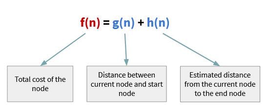
The algorithm will finally combine the actual cost from the start node -
g(n)- with the anticipated cost to the destination node -h(n)- and use the result to decide which node to examine next.
(Told you, it’s a simple addition expression!)😉
To find the best solution, you might have to use different heuristic functions according to the type of the problem.🎲 A* heuristic function, in essence, helps algorithms in making the right decision faster and more efficiently. 🚀 In fact, a heuristic function's core qualities 🔰 are Admissibility and Consistency.
However, creating these functions is a difficult task, and this is the fundamental problem we face in A* Algorithms.😩
But again, don't worry if all of this seems overwhelming too!😅 Let’s move on to the following section. It will undoubtedly ease your mind. 👇❄️
Behind the scenes of A* Search Algorithm
📌 Now that you know more about this algorithm let's see how it works behind the scenes with a step-by-step example. We will be using the same Undirected, Weighted Graph that we used for Dijkstra’s Algorithm.
💡Step 1: Inspecting the nearby nodes of the starting node A and calculate f(n)

💡Step 2: Analyze which f(n) is smaller and calculate f(n) for its neighbors
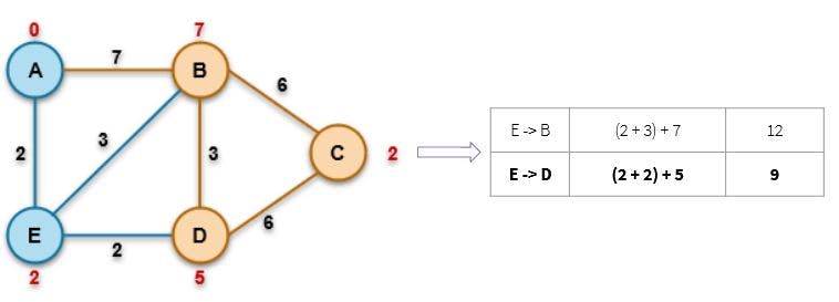
💡Step 3: Analyze which f(n) is smaller and calculate f(n) for the destination node
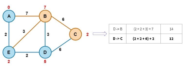
Tracing our paths now, the exact path that gives us the shortest distance between the nodes A and C is:
A -- E -- D -- C.
Implementation with Python
def aStarAlgo(start_node, stop_node):
        open_set = set(start_node)
        closed_set = set()
        g = {}  #store distance from starting node
        parents = {}  #contains an adjacency map of all nodes
        g[start_node] = 0
        parents[start_node] = start_node
        while len(open_set) > 0:
            n = None  #node with lowest f() is found
            for v in open_set:
                if n == None or g[v] + heuristic(v) < g[n] + heuristic(n):
                    n = v
            if n == stop_node or Graph_nodes[n] == None:
                pass
            else:
                for (m, weight) in get_neighbors(n):
                    if m not in open_set and m not in closed_set:
                        open_set.add(m)
                        parents[m] = n
                        g[m] = g[n] + weight
                    else:
                        if g[m] > g[n] + weight:
                            g[m] = g[n] + weight
                            parents[m] = n
                            if m in closed_set:
                                closed_set.remove(m)
                                open_set.add(m)
            if n == None:
                print('Path does not exist!')
                return None
            if n == stop_node:
                path = []
                while parents[n] != n:
                    path.append(n)
                    n = parents[n]
                path.append(start_node)
                path.reverse()
                print('Path found: {}'.format(path))
                return path
            open_set.remove(n)
            closed_set.add(n)
        print('Path does not exist!')
        return None

#function to return neighbor and its distance from the passed node
def get_neighbors(v):
    if v in Graph_nodes:
        return Graph_nodes[v]
    else:
        return None

#for simplicity we consider heuristic distances given and this function returns heuristic distance for all nodes
def heuristic(n):
        H_dist = {
            'A': 0,
            'B': 7,
            'C': 2,
            'D': 5,
            'E': 2,
        }
        return H_dist[n]

#Describe your graph here
Graph_nodes = {
    'B': [('A', 7), ('C', 6), ('D', 3), ('E', 3)],
    'A': [('B', 7), ('E', 2)],
    'C': [('B', 6), ('D', 6)],
    'D': [('B', 3), ('C', 6), ('E', 2)],
    'E': [('A', 2), ('B', 3), ('D', 2)]}
aStarAlgo('A', 'C')
Output: Path found: ['A', 'E', 'D', 'C']
Dijkstra's Shortest Path Algorithm vs. A* Search Algorithm
Coming towards the end, let us now get to compare both of these super-powerful algorithms that we just studied!👀
The first basis of comparison is the Time Complexities.
| Dijkstra’s Algorithm | A* Search Algorithm | Description | |
| Worst Time Complexity | O(E log V) | O(V) | V is the number of vertices |
| E is the total number of edges |
Note: The time complexity of the A* Algorithm depends heavily on the heuristic.
Firstly, we will talk about Dijkstra’s algorithm.
Dijkstra's key advantage is that it uses an uninformed algorithm.💪 This means it doesn't need to be informed of the destination node ahead of time.
✔️ You can utilize this functionality when you don't know anything about the graph and can't estimate the distance between each node and the goal.
When you have several target nodes, it comes in handy. Dijkstra often covers a vast portion of the graph since it selects the edges with the lowest cost at each step. This is particularly useful when you have numerous target nodes and aren't sure which one is the closest.
Now comes the A* algorithm.
If you ask what the best 2-D path-finder algorithm is, then the answer is A* Algorithm! 🌟 It is an intelligent algorithm that separates it from the other conventional algorithms.
People choose A* over Dijkstra’s Algorithm as Dijkstra’s Algorithm fails on the negative edge weights. 👎 Additionally, since it does a blind search, it wastes a lot of time while processing!🕗
📍 But, as every coin has two sides, people prefer Dijkstra's Algorithm in some circumstances since A* cannot be applied to graphs with many target nodes❗
This is because it has to be executed multiple times (one for each target node) to reach all of them.🔁
⚠️ Another main drawback of the A* Algorithm is the memory requirement.
It keeps all generated nodes in the memory, so it is not practical for various large-scale problems. ⛔
🔺 Another greatest challenge in selecting A* is the need for a good heuristic function. The time it takes to provide the heuristic must not cancel out any time savings in the process of path-finding. 🕜
That’s it!⭐ Now you know how these algorithms work behind the scenes and which one you would choose depending on the application.🚀
Happy reading!
I hope you enjoyed this article and found it helpful! 💯 For more such cool blogs and projects, check out our YouTube channel.👉
