Creating a simple neural network using TensorFlow

Want to build your first artificial neural network but do not know where to start?🤔 You might be surprised to learn that neural networks are not all that complex!🤩 You can learn all of the steps required by following this short lesson. Let us start with the fundamentals, shall we?🤗

What are Neural Networks?

Neural networks are designed for deep learning algorithms to function. In other words, they are just striving to produce accurate forecasts✔📈, as any different machine learning model.🤖 But what distinguishes them is their capacity to process massive amounts of data 📚 and predict the targets with great accuracy! 💯

So, let us see the definition of neural networks.

Artificial neural networks are a collection of nodes, inspired by brain neurons, that are linked together to form a network.

In general, a neural network consists of an input layer, one or more hidden layers, an output layer and is linked together 🔀 to give outputs. The activation function shown here is a hyperparameter that will be addressed later in the blog.

P and Q are input neurons in the above 👆 diagram, and w0 and w1 are the weights.

📍 It is important to note that w1 and w2 measure the strength 💪 of connections made to the center neuron, which sums(➕) up all inputs. Here, b is a constant known as the bias constant. This is what it looks like mathematically:

SUM = w1 * P + w2 * Q + b

📍 As long as the sum exceeds zero, the output is one or 'yes'; otherwise, it is zero or 'no.' Each input is linked with a weight in a neural network.

The steepness of the activation function rises 📈 as the weight increases. In other words, weight determines how quickly the activation function will fire 🔥, whereas bias is utilized to delay activation.

Like the intercept 📈 in a linear equation, bias is introduced to the equation. Hence, bias is a constant that aids the model to fit the provided data 📚 in the best possible way💯.

Implementing deep learning algorithms can be daunting👎, but thanks to Google's TensorFlow - which makes obtaining data📝, training models, serving predictions📊, and improving future outcomes more accessible🤩.

What is TensorFlow?

TensorFlow is a free and open-source framework built by the Google Brain team for numerical computing 🧮 and solving complex machine learning 🤖 problems. TensorFlow incorporates a wide variety of deep learning models and methods through its shared paradigm🔺. TensorFlow enables developers to construct dataflow graphs, which are data structures that represent how data flows across a graph or a set of processing nodes. Each node in the graph symbolizes a mathematical process, and each link or edge between nodes is a tensor, which is a multidimensional array.

Now, let us build our first neural network with TensorFlow.

We will be using a vehicle 🚗 detection dataset from Kaggle. This is a binary classification problem. The idea 💡 is to develop a model that can distinguish between pictures with and without cars 🚗. For the execution, Kaggle notebooks are used; you may alternatively use Google Colab.

Click here to download the dataset!

📍 The dataset consists of 8792 images of vehicles and 8968 images of non-vehicles. So, let us begin by importing the dataset:

import numpy as np
import pandas as pd

import os
for dirname, _, filenames in os.walk('/kaggle/input'):
    for filename in filenames:
        os.path.join(dirname, filename)

maindir = "../input/vehicle-detection-image-set/data"
os.listdir(maindir)

Output: ['vehicles', 'non-vehicles']

vehicle_dir = "../input/vehicle-detection-image-set/data/vehicles"
nonvehicle_dir = "../input/vehicle-detection-image-set/data/non-vehicles"
vehicle = os.listdir(maindir+"/vehicles")
non_vehicle = os.listdir(maindir+"/non-vehicles")
print(f"Number of Vehicle Images: {len(vehicle)}")
print(f"Number of Non Vehicle Images: {len(non_vehicle)}")

Output: Number of Vehicle Images: 8792 | Number of Non-Vehicle Images: 8968

📍 Let us print an image from vehicle_dir:

import cv2
import matplotlib.pyplot as plt
vehicle_img = np.random.choice(vehicle,5)
img = cv2.imread(vehicle_dir+'/'+vehicle_img[0])
img = cv2.cvtColor(img, cv2.COLOR_BGR2RGB)
plt.xlabel("Vehicle")
plt.tight_layout()
plt.imshow(img)
plt.show()

Output:

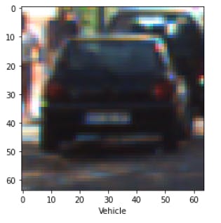
There are several open-source libraries for computer vision 🤖and image processing🎞. OpenCV is one of the largest. Using pictures and videos, it can recognize items, people, and even the handwriting of a human being.

When the user calls cv2.imread(), an image is read from a file. Among the programming languages supported by OpenCV are Python, C++, and Java.

📍 We will also check an image in the nonvehicle_dir:

import cv2
import matplotlib.pyplot as plt
nonvehicle_img = np.random.choice(non_vehicle,5)
img = cv2.imread(nonvehicle_dir+'/'+nonvehicle_img[0])
img = cv2.cvtColor(img, cv2.COLOR_BGR2RGB)
plt.xlabel("Non-Vehicle")
plt.tight_layout()
plt.imshow(img)
plt.show()

Output:

📍 We now split the data into train and test datasets:

train = []
test = []
import tqdm
from tensorflow.keras.preprocessing import image

for i in tqdm.tqdm(vehicle):
    img = cv2.imread(vehicle_dir+'/'+ i)
    img = cv2.resize(img,(150,150))
    train.append(img)
    test.append("Vehicle")

for i in tqdm.tqdm(non_vehicle1):
    img = cv2.imread(nonvehicle_dir+'/'+ i)
    img = cv2.resize(img,(150,150))
    train.append(img)
    test.append("Non Vehicle")

Output:

📍 We can create console line progress bars and GUI progress bars with the help of the tqdm library. We use these progress indicators to check ✔ if we are getting stuck someplace and work on it right away 💯.

train = np.array(train)
test = np.array(test)
train.shape,test.shape

Output: ((17584, 150, 150, 3), (17584,))

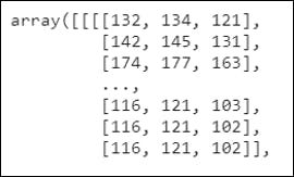
📍 The train dataset contains arrays of different images, whereas the test dataset consists of the labels for each respective image.

📍 Let us check the train and test datasets:

train[:2]

Output:

test

Output: array(['Vehicle', 'Vehicle', 'Vehicle', ..., 'Non Vehicle', 'Non Vehicle', 'Non Vehicle'], dtype='<U11')

📍 The test data, unfortunately, consists of the string labels. First, we have to convert it into numeric data 🔢; for instance, vehicles will be labeled as 1, and non-vehicles will be labeled as 0.

from sklearn.preprocessing import LabelEncoder
le = LabelEncoder()
test= le.fit_transform(test)

test

Output: array( [ 1, 1, 1, . . . . , 0, 0, 0 ] )

📍 Now this will make our life easier!🤗

📍 The next step involves splitting the train dataset into x_train, y_train, and the test dataset into x_test, y_test. But before that, we need to shuffle the training and testing datasets. Shuffle is nothing more than rearranging the items of an array.

from sklearn.utils import shuffle
train,test = shuffle(train, test)

from sklearn.model_selection import train_test_split
x_train,x_test,y_train,y_test = train_test_split(train,test,test_size=0.2,random_state = 50)

Model Training:

import tensorflow as tf
model = tf.keras.models.Sequential()

📍 The Sequential API is the simplest model to construct and run in Keras. A sequential model enables us to build models layer by layer.

📍 An important thing to note is that right now; the images are in a multidimensional array. We want them to be flat rather than n-dimensional. If we were to use something more powerful like CNN, we might not require it. But in this case, we definitely want to flatten it. For this, we can use one of the layers that are in-built keras.

model.add(tf.keras.layers.Flatten())

📍 The following essential steps involve building the layers. We will create five layers to obtain the result.

model.add(tf.keras.layers.Dense(128, activation = tf.nn.relu))
model.add(tf.keras.layers.Dense(64, activation = tf.nn.relu))
model.add(tf.keras.layers.Dense(32, activation = tf.nn.relu))
model.add(tf.keras.layers.Dense(16, activation = tf.nn.relu))

model.add(tf.keras.layers.Dense(2, activation = tf.nn.softmax))  # Output Layer

📍 The next most important thing is to decide the number of neurons in the hidden layers. We typically use systematic experimentation to determine what works best for our particular dataset. Typically, the number of hidden neurons should decrease in succeeding layers as we move closer to the pattern and identify the target labels.

📍 I have taken 128 neurons for the first layer, and for the subsequent layers, I have used 64, 32, and 16 neurons, respectively. You are free to experiment around these parameters. The output layer always consists of the number of classifications; in our case, it is 2. Sometimes, the last layer of a classification network is activated using softmax and the output is a probability distribution of the targets.

📍 An activation function is utilized for the internal processing of a neuron. The activation function of a node describes the output of that node, given input or collection of inputs. We already know that an artificial neural network computes the weighted sum of its inputs and then adds a bias. Now, the value of net output might range from -Inf to +Inf. The neuron does not understand how to bind the value and so cannot determine the firing pattern 🔥. Thus, the activation function determines whether or not a neuron should be activated.

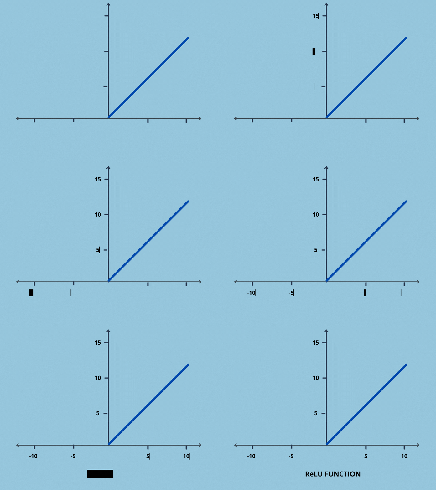
📍 There are many activation functions like sigmoid, tanh. 'Rectified Linear' or relu is one of the activation functions utilized in deep learning models. If it gets any negative input, it returns 0, but if it receives any positive input, it returns that value. As a result, it may be written as:

f (x) = max (0, x)

model.compile(optimizer = 'adam',
               loss = 'categorical_crossentropy',
               metrics = ['accuracy'])

📍 We will use adam as our optimization algorithm for iteratively updating the weights.

📍 Epochs - are the number of times our training dataset will pass through our neural network and are defined as a hyperparameter (a parameter whose value is used to regulate the learning process).

📍 Categorical_crossentropy - Each predicted value is compared to the actual output of 0 or 1, and a score/loss is computed depending on how much it differs from the true value.

model.fit(x_train, y_train, epochs = 10)

Output:

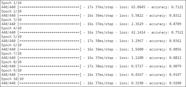
📍 You can notice that with each layer, the loss is decreasing, and the model's accuracy is increasing. The highest accuracy reached was approximately92%.

📍 We can also evaluate this by:

val_loss, val_acc = model.evaluate(x_test, y_test)
print(val_loss, val_acc)

Output: 110/110 [==============================] - 1s 12ms/step - loss: 0.2342 - accuracy: 0.9338

Predicting:

predictions = model.predict([x_test])
print(predictions)

Output: [[8.3872803e-02 9.1612726e-01] [7.1111350e-07 9.9999928e-01] [1.9085113e-03 9.9809152e-01] ... [9.9999988e-01 1.5221100e-07] [7.8120285e-01 2.1879715e-01] [3.9260790e-08 1.0000000e+00]]

📍 Wow, that looks like a mess!😵 Let us try to simplify it:

y_pred = model.predict(x_test)
y_pred = np.argmax(y_pred,axis=1)
y_pred[:15]

Output: array([1, 1, 1, 0, 1, 0, 1, 1, 1, 1, 1, 1, 0, 0, 1])

📍 We can also crosscheck✔ the actual values vs. the predicted values:

y_test = np.argmax(y_test,axis=1)
y_test[:15]

Output: array([1, 1, 1, 0, 1, 0, 1, 1, 1, 1, 1, 1, 0, 0, 1])

📍 That’s amazing; the values are almost matching! To get a better look, try:

plt.figure(figsize=(12,9))
sample_idx = np.random.choice(range(len(x_test)))
plt.subplot(2,5,i+1)
plt.imshow(x_test[sample_idx])
plt.xlabel(f"Actual: {y_test[sample_idx]}" )
plt.xlabel(f"Predicted: {y_pred[sample_idx]}")
plt.tight_layout()
plt.show()

Output:

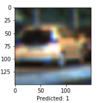
print("y_test value: ",y_test[sample_idx])
print("y_pred value: ",y_pred[sample_idx])

Output: y_test value: 1 | y_pred value: 1

Kudos! You have built your first neural network using TensorFlow!

We hope you liked and found this blog useful!🤩Check out our other blogs below! Also, subscribe to our YouTube channel for more great videos and live projects⭐.